4. Appendix of additional (secondary) code.

• Testing utility functions

• Secondary numerical exploratioins

import numpy as np
import pandas as pd
import matplotlib.pyplot as plt
from matplotlib.patches import Ellipse
import matplotlib.transforms as transforms
from collections import namedtuple
from scipy import linalg
import utils

4.1. Is my covariance ellipse implementation correct?

Compare my implementation to matplotlib’s implementation.

# The matplotlib implementation.
def confidence_ellipse(x, y, ax, n_std=3.0, facecolor='none', **kwargs):
    if x.size != y.size:
        raise ValueError("x and y must be the same size")

    cov = np.cov(x, y)
    pearson = cov[0, 1]/np.sqrt(cov[0, 0] * cov[1, 1])
    # Using a special case to obtain the eigenvalues of this
    # two-dimensional dataset.
    ell_radius_x = np.sqrt(1 + pearson)
    ell_radius_y = np.sqrt(1 - pearson)
    ellipse = Ellipse((0, 0), width=ell_radius_x * 2, height=ell_radius_y * 2,
                      facecolor=facecolor, **kwargs)

    # Calculating the standard deviation of x from
    # the squareroot of the variance and multiplying
    # with the given number of standard deviations.
    scale_x = np.sqrt(cov[0, 0]) * n_std
    mean_x = np.mean(x)

    # calculating the standard deviation of y ...
    scale_y = np.sqrt(cov[1, 1]) * n_std
    mean_y = np.mean(y)

    transf = transforms.Affine2D() \
        .rotate_deg(45) \
        .scale(scale_x, scale_y) \
        .translate(mean_x, mean_y)

    ellipse.set_transform(transf + ax.transData)
    return ax.add_patch(ellipse)

# Visually show both implementations produce the same confidence ellipse
mu = np.array([1,2])
S = np.array([[2., 1.9], [1.9, 2]])

data = np.random.multivariate_normal(mu, S, size=5000)
x = data[:,0]
y = data[:,1]

fig, ax = plt.subplots()
ax.scatter(x,y,s=1)
confidence_ellipse(x, y, ax, n_std=3.0, edgecolor='red', label='Matplotlib implementation')
utils.plot_covar_ellipse(S, mu, mult=3.0, label='My implementation')
plt.legend()
plt.show()

print('My implementation matches that of matplotlib\'s example code')

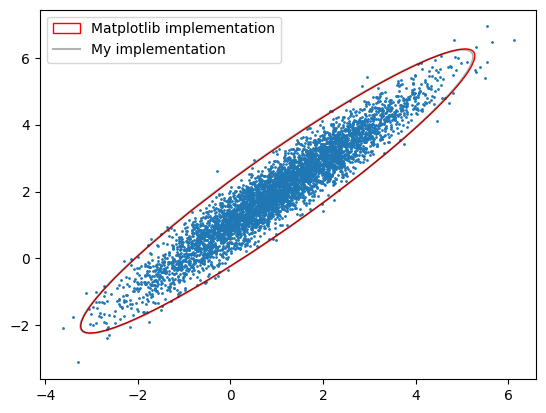
My implementation matches that of matplotlib's example code

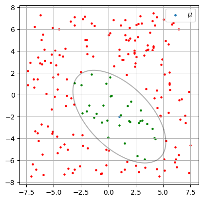
4.2. Is a given point inside a covariance ellipse?

Demonstrate my utility function that determines if a given 2D point \(\vec{p}\) is in the closure of a given confidence ellipse centered at \(\mu\) with semi-major axis \(r_1\), semi-minor axis \(r_2\). (\(r_1 = \alpha \sqrt{\lambda_1}\) and \(r_2 = \alpha \sqrt{\lambda_2}\) where \(\alpha\) scales the number of standard deviations we wish the ellipse to visualize)

If

\(\left(\frac{cos(\theta)(p_x-\mu_x)+sin(\theta)(p_y-\mu_y)}{r_1}\right)^2 + \left(\frac{sin(\theta)(p_x-\mu_x)-cos(\theta)(p_y-\mu_y)}{r_2}\right)^2 \leq 1\)

Then \(\vec{p}\) is inside the ellipse. [cov]

# Define our ellipse
mu = np.array([1,-2])
S = np.array([[2., -1.1], [-1.1, 2]])

# Generate uniform random test points
x_lim = 15.0
points = np.random.random((200, 2)) * x_lim - np.array([x_lim/2, x_lim/2])

fig, ax = plt.subplots()
ax.set_aspect('equal')
ax.scatter(mu[0], mu[1] , s=6, label=r'$\mu$')
utils.plot_covar_ellipse(S, mu, mult=3.0)

# Test if our test points are inside the ellipse
for p in points:
    color = 'green' if utils.ellipse_contains(p, mu, S, n_std=3) else 'red'
    ax.scatter(p[0], p[1], s=5, color=color)

#assert ellipse_contains(p, mu, S, n_std=3)
plt.legend()
plt.grid()
plt.show()

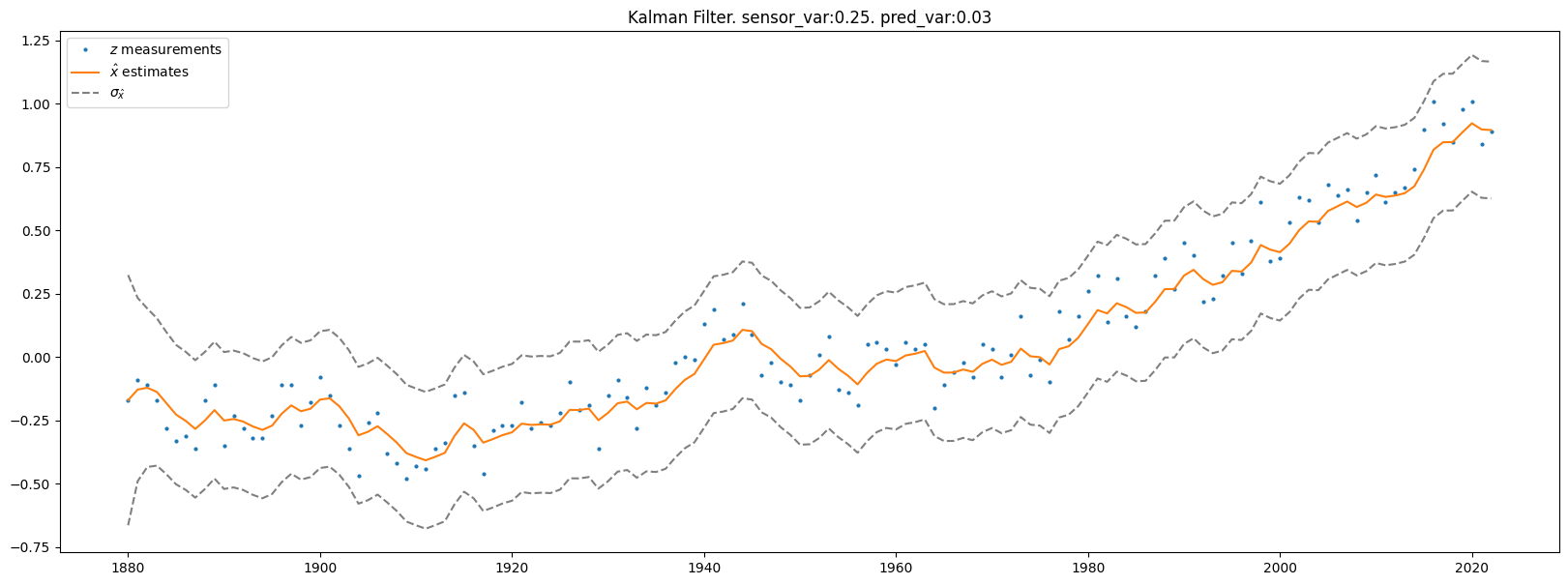
4.3. Bayesian Style Implementation of 1D Kalman Filter

# Named tuples to represent gaussian distributions
Gauss = namedtuple('Gauss', 'mean var')

df = pd.read_csv('temp_anomalies.csv')
pred_var = 0.03
sensor_var = 0.25

# Measurements
zs = df.no_smoothing

# Initialize system and filter state
# Prior
x_hat = Gauss(zs[0], 10) # Initialize estimate to first measurement value

x_hats = np.full(len(zs), np.nan)
x_hat_vars = np.full(len(zs), np.nan)

for i in range(len(zs)):
    z = zs[i]
    
    # Prediction step - via process model
    dx = Gauss(0, pred_var)
    prior = Gauss(x_hat.mean + dx.mean, x_hat.var + dx.var)
    
    # Update (correct the prediction - from prior to posterior)
    l = Gauss(z, sensor_var) # Likelihood of measurement
    post_mean = (prior.var * l.mean + l.var * prior.mean)/(prior.var + l.var)
    post_var = (prior.var * l.var) / (prior.var + l.var)
    x_hat = Gauss(post_mean, post_var)
    x_hats[i] = x_hat.mean
    x_hat_vars[i] = x_hat.var
    
    # Posterior becomes next iterations prior
    prior = x_hat
    
plt.rcParams["figure.figsize"] = (20,7)
plt.plot(df.year, df.no_smoothing, marker='o', linestyle='none', markersize=2, label=r'$z$ measurements')
plt.plot(df.year, x_hats, label=r'$\hat{x}$ estimates')
plt.plot(df.year, x_hats + np.sqrt(x_hat_vars), linestyle='dashed', color='gray', label='$\sigma_{\hat{x}}$')
plt.plot(df.year, x_hats - np.sqrt(x_hat_vars), linestyle='dashed', color='gray')
plt.title(f'Kalman Filter. sensor_var:{sensor_var}. pred_var:{pred_var}')
plt.legend()
plt.show()

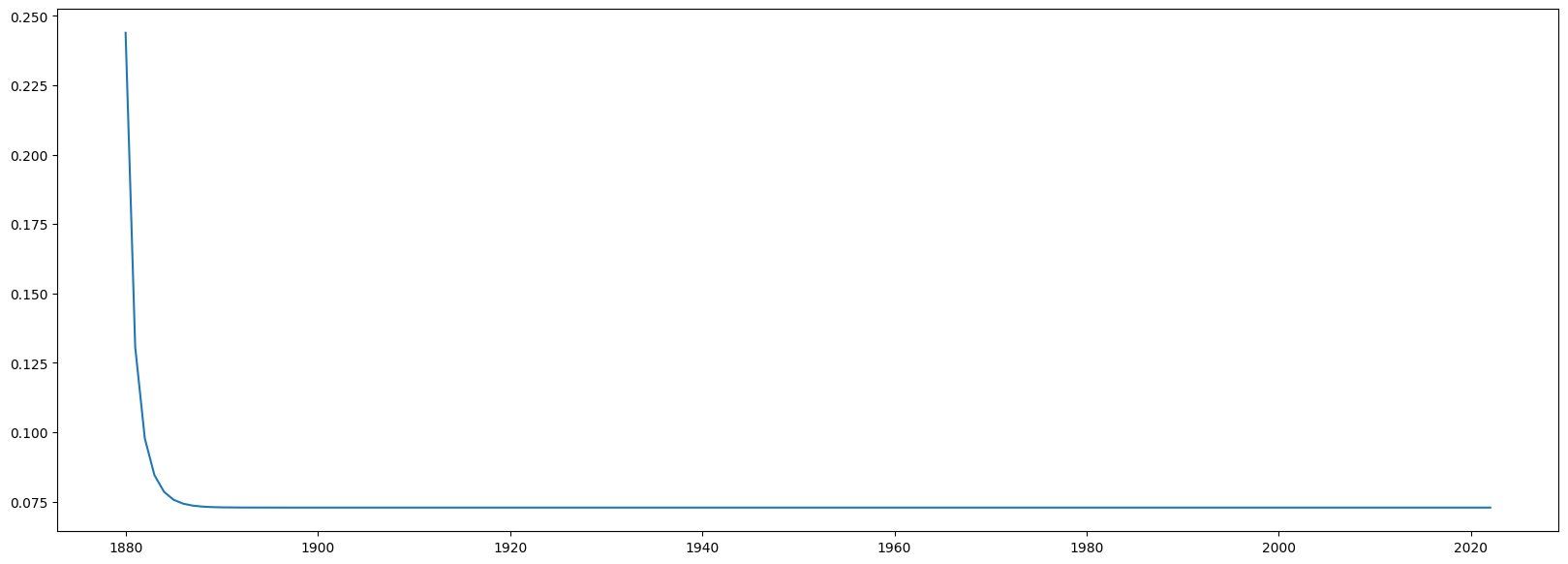
print('Estimate variance')
plt.plot(df.year, x_hat_vars)
plt.show()

Estimate variance

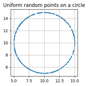
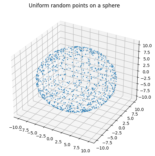
4.4. Muller Algorithm

The Muller algorithm is a method to efficiently generate random samples on the surface of a (\(d-1\))-sphere. The algorithm is based on the fact that the joint distribution of \(d\) normally distributed RVs can be mapped to vectors that are uniformly distributed along the surface of a (\(d-1\))-sphere. [Rob19]

# Testing Muller algorithm to generate uniform points on a (d-1)-sphere

# d=2: Circle (d-1 = 1 degree of freedom)
figure, axes = plt.subplots(1, figsize=(3,3)) 
axes.set_aspect(1)
r = 5
d = 2
v0 = np.zeros(d) + 10
num_points = 500
points = np.full((num_points,d), np.nan)
for i in range(num_points):
    points[i] = utils.random_point_on_dsphere(r=r, d=d, v0=v0)
axes.scatter(points[:,0], points[:,1], s=2)
plt.title('Uniform random points on a circle')
plt.grid()
plt.show()

# d=3: Sphere (d-1 = 2 degrees of freedom)
fig = plt.figure(figsize=(6,6))
ax = fig.add_subplot(projection='3d')
r = 10
d = 3
v0 = np.zeros(d)
num_points = 1000 # Num points
points = np.full((num_points,d), np.nan)
for i in range(num_points):
    points[i] = utils.random_point_on_dsphere(r=r, d=d, v0=v0)
ax.scatter(points[:,0], points[:,1], points[:,2], s=2)
plt.title('Uniform random points on a sphere')
plt.show()