1. Writeup

I summarize my explorations and findings in this Writeup section.

1.1. The 1D Kalman Filter

Here we implement the 1D Kalman filter and apply it to a simple problem involving global temperature data.

1.1.1. Implementation

As in [You11] (Chapter 4.4, moving body example) we implement the linear Kalman filter to estimate a single state variable over time.

The code for that implementation is in Section 2.2.1.

1.1.2. Demonstration on temperature data

As Young points out, there is a relationship between the filtering problem and regression. We can transform a regression problem into the filtering problem, then apply the Kalman Filter.

To demonstrate this, take the following data set from NASA [nas], which depicts the annual global average temperature as compared to a baseline temperature (the average temperature over the period of 1951 to 1980):

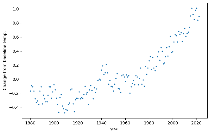
There is clearly an upward trend, but the data is noisy - from one year to the next the annual temperature average may go up or down. Furthermore, the upward trend appears nonlinear. How can we determine the trend from the noise?

We may transform this into filtering problem in a few ways:

1. Imagine the temperature is a noisy process and we have perfect measurements.

2. Imagine the temperature is fully deterministic process and we have noisy measurements.

3. Imagine the both the temperature process and our measurements have noise.

Then our Kalman filter estimate will be a regression of this temperature data.

Let’s go with option 3. If we design our process to assume a constant temperature (\(x(k) = x(k-1) + \eta(k)\)), then choose measurement noise variance \(R\) = 0.5 and process noise \(Q\) = 0.05, we get the following filter output:

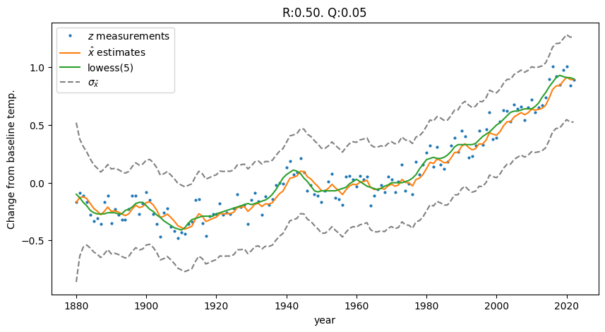
Fig. 1.1 The kalman-estimated temperature trend approximates the lowess regression of the noisy temperature data. Code in Section 2.2.1.

1.1.3. A linear kalman filter applied to non-linear data?

Why was our linear-process-model Kalman Filter able to produce a non-linear regression? Even though we defined a constant temperature process, it is still a stochastic process with some non-zero noise \(\vec{\eta}(k) \sim \mathcal{N}(0, Q)\). That uncertainty in the process-based predictions allows the measurements to pull the estimates upwards during the update steps.

The way we tune \(Q\) and \(R\) impacts this behavior. The two other extremes of parameter tuning (options 1 and 2 listed above) produce the following filter outputs:

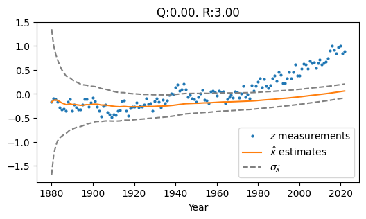
Fig. 1.2 Low Q, High R

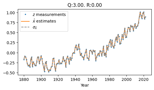
Fig. 1.3 High Q, Low R

Fig. 1.2 Shows Low Q and High R (\(Q\) = 0.0, \(R\) = 3.0). The result is an estimate that lags behind the upward trend of the measurements, because the constant-temp process model’s predictions are weighted more heavily than the measurements.

Fig. 1.3 Shows High Q and Low R (\(Q\) = 3.0, \(R\) = 0.0). The result is a jagged estimate that hugs the data points tightly because our filter assumes no measurement noise.

The code that generated both the above figures is in Section 2.2.3.

1.1.4. Behavior in the presence of data gaps

My implementation replicates Young’s illustration of how the filter estimate’s variance \(P\) grows over a period of missing data.

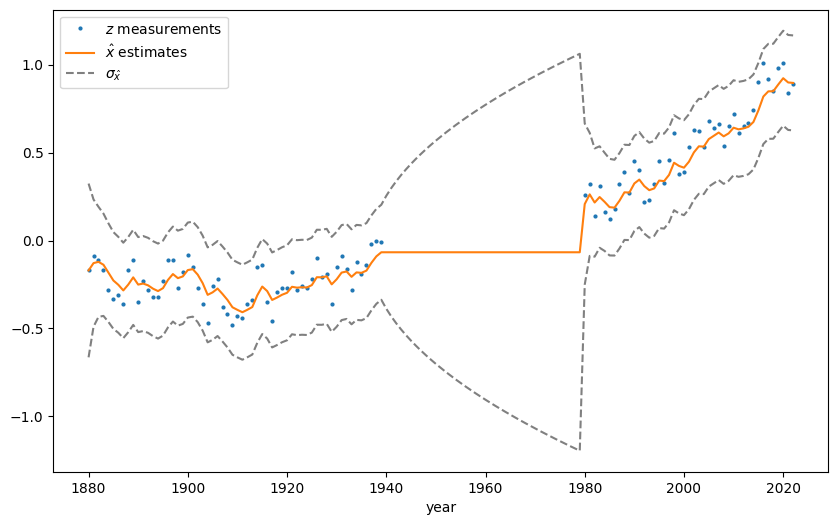
Fig. 1.4 The \(1 \sigma\) error bounds depicting \(P(k)\) grows over a period of missing measurement data, before contracting quickly once new data points come in. Code in Section 2.2.2.

1.2. The Multivariate Kalman Filter

1.2.1. Implementation and synthesis of input data

I implemented a multivariate Kalman Filter (Section 2.4.3) and synthesized a true 6-dimensional data series \(\vec{x}(k)\) for a moving object under constant acceleration and its measurements \(\vec{z}(k)\) (Section 2.4.1).

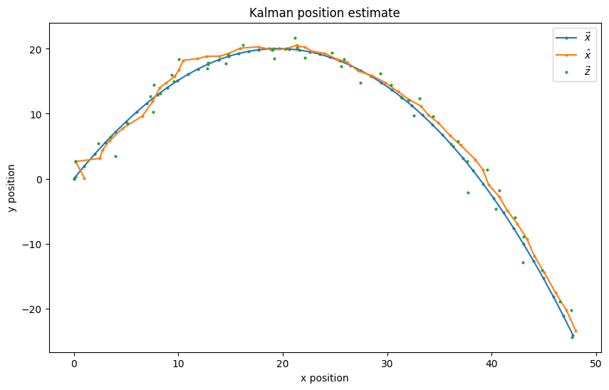
Fig. 1.5 The filter produces a position estimate that is convincingly close to the true state’s postition.

If we pull out the position, velocity, and acceleration estimates and covariance matrices from \(\vec{x}(k)\) and \(P(k)\) we can visualize them separately (Section 2.4.4):

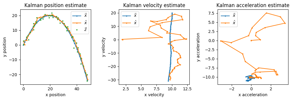
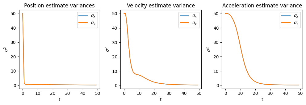
Fig. 1.6 Estimates and their respective variances over time.

We see the position estimate quickly converges close to the true position, and similarly the position estimate’s variance \(\begin{bmatrix} \sigma_{x} & 0 \\ 0 & \sigma_{y} \end{bmatrix}\) rapidly reduces in magnitude. Fig. 1.6 shows the steep reduction in \(\sigma_{x}\) and \(\sigma_{y}\), and that a similar convergence plays out for the velocity estimates/variance at a slower rate, and for acceleration at a slower rate still.

1.2.2. Accuracy Metrics

I primarily explore 2 methods of quantifying accuracy:

1. Normalized Estimated Error Squared (NEES).

2. \(3 \sigma\) Membership Accuracy Score: The ratio of estimates \(\hat{x}(k)\) whose \(3 \sigma\) covariance ellipses of \(P(k)\) contain the true state \(\vec{x}(k)\).

1.2.2.1. Normalized Estimated Error Squared (NEES)

NEES is a standard way of evaluating the accuracy of the Kalman filter when the true state series \(\vec{x}(k)\) is known (as is the case here). Details of my implementation and exploration are in Section 2.4.6.1.

1.2.2.2. \(3 \sigma\) Membership Accuracy Score

I implemented an intuitive and simple way of quantifying the accuracy of the Kalman filter’s estimates.

The score works as follows. For each estimate \(\hat{x}(k)\), check if the associated true state point \(\vec{x}(k)\) falls within the \(3\sigma\) covariance ellipse for \(P(k)\). Then simply compute the ratio of estimates for which \(\vec{x}(k)\) is a member of \(\hat{x}(k)\)’s ellipse out of all estimates. Implementation in Section 2.4.6.2.

Here’s a visualized example, where the Kalman filter’s \(3\sigma\) membership accuracy score is 0.8:

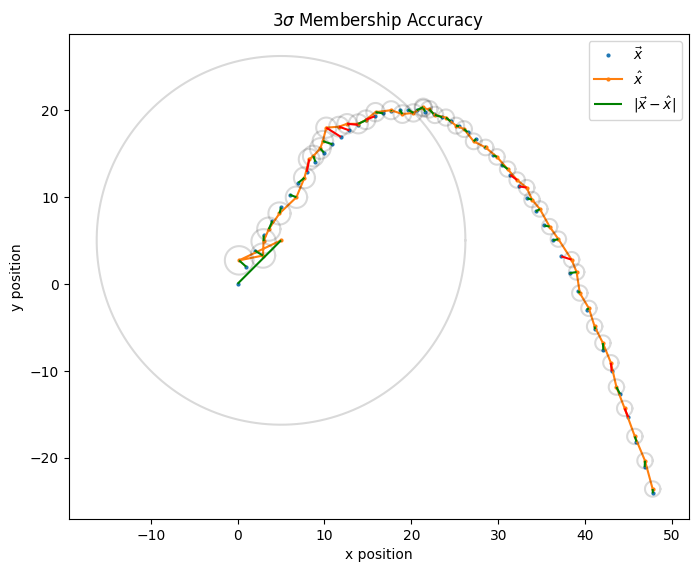
Fig. 1.7 Each (\(\hat{x}(k)\), \(\vec{x}(k)\)) pair is connected by a line segment, which is colored green if \(\vec{x}(k)\) is a member of \(\hat{x}(k)\)’s \(3\sigma\) ellipse and red otherwise.

Note: This score only useful for relative comparisons between filter runs on the same data set, which is primarily what I’m doing here. Furthermore, the scalar nature of the score loses information about the filter performance, such as the relative speed at which the residual magnitudes \(|\vec{x}(k)-\hat{x}(k)|\) converge.

1.2.3. Performance

Our filter’s behavior is dependent on our choice of a few parameters, including an initial state estimate \(\hat{x}(0)\), initial estimate covariance \(P(0)\), and covariances \(R\), and \(Q\). How sensitive is the filter’s accuracy to the perturbations to those parameters?

1.2.3.1. Initial state estimate perturbation

I used Monte Carlo methods to explore the relationship between initial state estimate perturbations and the filter accuracy distribution. As perturbations to the initial state guess \(\hat{x}(0)\) increase, the sample mean of both accuracy metrics decreases and variance increases:

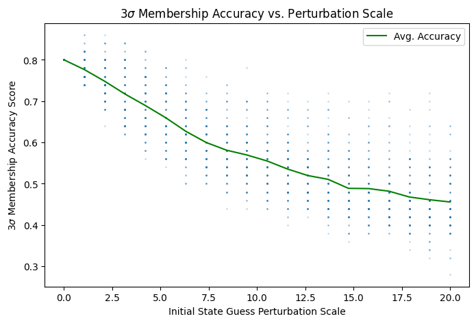
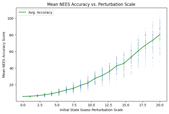
Fig. 1.8 Increasing average NEES scores means lower overall estimate accuracy.

The code that produced both figures above is in Section 2.4.7. Random perturbation vectors were generated on \((d-1)\)-balls of increasing radii via the Muller method Section 4.4).

1.2.3.2. \(Q\),\(R\) perturbation from their true values.

What if we didn’t know the true values of \(Q\) and \(R\) and needed to approximate or guess their values? How does the filter’s accuracy change as a function of a perturbations of \(Q\) and \(R\) from their true values?

In Section 2.4.8 I numerically explore a sub-section of the (\(Q\),\(R\)) parameter space and produce accuracy surfaces (for both metrics):

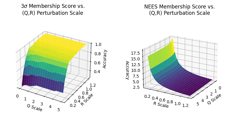
The result is that in scaling process noise \(Q\) has little impact on the filter’s estimation accuracy with our data set, while scaling measurement noise \(R\) has relatively high impact. As we increase R’s values from \(0\) to \(0.6\) of \(R*\) (the true measurement noise) we get a rapid increase in accuracy, which then converges asymptotically to a stable high accuracy value for larger scaling factors.

1.3. Conclusion

I have implemented the univariate and multivariate Kalman Filter, implemented 2 methods to evaluate its accuracy, and conducted a number of numerical explorations including applying the filter to perform regression on global temperature data and evaluating the accuracy of the multivariate filter’s estimates on a synthetic data set in response to perturbing filter parameters.

The lower-level details of my explorations, including a number of explorations I did not feel warranted inclusion in the write up, may be found in the Code section below and in the Secondary Code Appendix.

2. Code

Below are the details of my analysis, including code implementation and low-level explanations.

import numpy as np
import pandas as pd
import pandas as pd
import matplotlib.pyplot as plt
from matplotlib import collections as mc
from importlib import reload
from scipy.stats import chi2
from myst_nb import glue
import utils
reload(utils)

rng = np.random.default_rng(seed=1)
from IPython.core.debugger import set_trace

2.1. Global Temp Anomaly Data

df = pd.read_csv('temp_anomalies.csv')
fig, ax = plt.subplots(figsize=(8,5))
plt.plot(df.year, df.no_smoothing, marker='o', linestyle='none', markersize=2)
plt.xlabel('year')
plt.ylabel('Change from baseline temp.')
#plt.show()
glue("global_temp_data", fig, display=False)

2.2. The 1D Kalman Filter

2.2.1. Implementation

# Run the kalman filter algorithm on a series of observations and return
# the estimated state series
def kalman_1d(zs, R, Q, P_0, x_0):
    """
    Args:
        zs: Measurement series. An Nx1 array.
        R: Measurement noise variance.
        Q: Process noise variance
        P: Prior (prediction) variance.
    """
    # Initialize system and filter state
    xs = np.full(len(zs), np.nan)
    Ps = np.full(len(zs), np.nan)
    
    # Prior
    P = P_0
    x = x_0

    # TODO: Should we exclude prediction calculation for first iteration?
    for i in range(len(zs)):
        # PREDICT STEP - Process model update
        # dx = Gauss(0, Q)
        x = x + 0 # Prediction mean
        P = P + Q # Prediction var

        # UPDATE STEP (if there is a measurement at this timestep)
        if not np.isnan(zs[i]):
            resid = zs[i] - x

            # Kalman Gain
            K = P / (P + R)

            # Posterior: Use kalman gain to scale the residual between prediction and measurement
            x = x + K * resid
            P = (1 - K) * P

        # Save results
        xs[i] = x
        Ps[i] = P
        
    return xs, Ps

# Configure and run the filter
R = 0.5 # Measurement variance
Q = 0.05 # Process noise variance
glue('kalman_temp_R', R)
glue('kalman_temp_Q', Q)
zs = df.no_smoothing # Measurements
P_0 = 10
x_0 = zs[0]
xs, Ps = kalman_1d(zs, R, Q, P_0, x_0)

# Plot
fig, ax = plt.subplots(1, figsize=(10,5))
plt.plot(df.year, zs, marker='o', linestyle='none', markersize=2, label=r'$z$ measurements')
plt.plot(df.year, xs, label=r'$\hat{x}$ estimates')
plt.plot(df.year, df.lowess_5, label=r'lowess(5)')
plt.plot(df.year, xs + np.sqrt(Ps), linestyle='dashed', color='gray', label='$\sigma_{\hat{x}}$')
plt.plot(df.year, xs - np.sqrt(Ps), linestyle='dashed', color='gray')
plt.title(f'R:{R:.02f}. Q:{Q:.02f}')
plt.xlabel('year')
plt.ylabel('Change from baseline temp.')
plt.legend()
plt.show()
glue("global_temp_kalman", fig, display=False)

0.5

0.05

2.2.2. Exploring how the kalman filter behaves with data gaps

R = 0.25 # Measurement variance
Q = 0.03 # Process noise variance
zs = df.no_smoothing.to_numpy() # Measurements

# Define an data gap interval
start = 60 # Years beyond 1880
end = 100
gap_zs = np.copy(zs)
gap_zs[start:end] = np.nan
t = df.year.to_numpy()

fig, ax = plt.subplots(1, figsize=(10,6))
xs, Ps = kalman_1d(gap_zs, R, Q, P_0, x_0)
plt.plot(t, gap_zs, marker='o', linestyle='none', markersize=2, label=r'$z$ measurements')
plt.plot(t, xs, label=r'$\hat{x}$ estimates')
plt.plot(t, xs + np.sqrt(Ps), linestyle='dashed', color='gray', label='$\sigma_{\hat{x}}$')
plt.plot(t, xs - np.sqrt(Ps), linestyle='dashed', color='gray')
plt.xlabel('year')
plt.legend()
plt.show()
glue("kt_data_gap", fig, display=False)

2.2.3. Exploring the parameter space of \(Q\) x \(R\)

Illustrating how the measurement noise covariance \(R\), and process noise covariance is \(Q\) affect the behavior of the 1D Kalman filter.

def plot_temp_kalman_for_QR(Q, R, ax):
    P_0 = 10
    x_0 = zs[0]
    xs, Ps = kalman_1d(zs, R, Q, P_0, x_0)
    ax.plot(df.year, zs, marker='o', linestyle='none', markersize=2, label=r'$z$ measurements')
    ax.plot(df.year, xs, label=r'$\hat{x}$ estimates')
    ax.plot(df.year, xs + np.sqrt(Ps), linestyle='dashed', color='gray', label='$\sigma_{\hat{x}}$')
    ax.plot(df.year, xs - np.sqrt(Ps), linestyle='dashed', color='gray')
    ax.set_title(f'Q:{Q:.02f}. R:{R:.02f}')
    ax.set_xlabel('Year')
    ax.legend()

# Low Q, High R
Q, R = 0.0, 3.0
glue('kt_lqhr_Q', Q, display=False)
glue('kt_lqhr_R', R, display=False)
fig, ax = plt.subplots(figsize=(6,3))
plot_temp_kalman_for_QR(Q, R, ax)
glue("kt_lqhr_fig", fig, display=False)

# High Q, Low R
Q, R = 3.0, 0.0
glue('kt_hqlr_Q', Q, display=False)
glue('kt_hqlr_R', R, display=False)
fig, ax = plt.subplots(figsize=(6,3))
plot_temp_kalman_for_QR(Q, R, ax)
glue("kt_hqlr_fig", fig, display=False)

2.3. The Bayesian Intuition underlying the Kalman Filter

In his excellent exploration of the Kalman Filter [Lab], Roger Labbe illustrates the Bayesian intuition underlying the Kalman filter algorithm. I have implemented the Bayesian approach Section 4.3, and show it has the same result as the traditional implementation.

2.4. Multidimensional Kalman Filter (for a Process With Constant Acceleration)

In this section I synthesize data for a object moving in 2 dimensions under a constant acceleration (due to gravity), then apply a multidimensional Kalman filter and analyze the filter’s output and accuracy.

2.4.1. Synthesizing true state \(\vec{x}(k)\)

We will track the following 6-dimensional state vector: \(\vec{x} = \begin{bmatrix} x & \dot{x} & \ddot{x} & y & \dot{y} & \ddot{y}\end{bmatrix}^T\)

Let’s start by defining a deterministic process model (simple Newtonian motion under constant acceleration) for state \(\vec{x}(k)\) as:

\[\begin{split} \vec{x}(k) = \begin{bmatrix} x(k) \\ \dot{x}(k) \\ \ddot{x}(k) \\ y(k) \\ \dot{y}(k) \\ \ddot{y}(k) \\ \end{bmatrix} = \begin{bmatrix} 1 & \Delta t & \frac{1}{2}(\Delta t)^2 & 0 & 0 & 0 \\ 0 & 1 & \Delta t & 0 & 0 & 0 \\ 0 & 0 & 1 & 0 & 0 & 0 \\ 0 & 0 & 0 & 1 & \Delta t & \frac{1}{2}(\Delta t)^2 \\ 0 & 0 & 0 & 0 & 1 & \Delta t \\ 0 & 0 & 0 & 0 & 0 & 1 \\ \end{bmatrix} \begin{bmatrix} x(k-1) \\ \dot{x}(k-1) \\ \ddot{x}(k-1) \\ y(k-1) \\ \dot{y}(k-1) \\ \ddot{y}(k-1) \\ \end{bmatrix} = F \vec{x}(k-1) \end{split}\]

Where \(F\) is our transition matrix, \(\vec{x}(k-1)\) is the state at the previous time step, and \(\Delta t\) is the length of the time step.

Note that this implies constant acceleration in both dimensions. We’ll set our initial acceleration vector as acceleration due to gravity: \(\begin{bmatrix} \ddot{x} & \ddot{y} \end{bmatrix}^T = \begin{bmatrix} 0 & -9.81 \end{bmatrix}^T \)

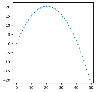
Now let’s simulate the trajectory of our deterministic process \(\vec{x}(k)\) over a period of time:

# Simulation config

# Timestep
dt = 0.1

# Number of seconds of simulation
T = 5
N = T / dt
assert N.is_integer()
N = int(N)

print(f'Simulating {T:.02f} seconds. {N} timesteps')

Simulating 5.00 seconds. 50 timesteps

# Initial position
x_0, y_0 = [0., 0]

# Initial velocity
vx_0, vy_0 = [10., 20]

# Initial (constant) acceleration
ax_0, ay_0 = [0, -9.81]

# Initial state
n = 6 # State dimensionality
x0 = np.array([x_0, vx_0, ax_0, y_0, vy_0, ay_0])

# Transition matrix
F = np.array([
    [1., dt, 0.5*dt**2, 0, 0, 0],
    [0, 1, dt, 0, 0, 0],
    [0, 0, 1, 0, 0, 0],
    [0, 0, 0, 1, dt, 0.5*dt**2],
    [0, 0, 0, 0, 1, dt], 
    [0, 0, 0, 0, 0, 1],
])

# Results matrix. Each row is the state for one timestep
xs = np.full((N, n), np.nan)
xs[0,:] = x0

for k in range(1, N):
    xs[k, :] = F @ xs[k-1, :]
    
plt.rcParams["figure.figsize"] = (4,4)
plt.plot(xs[:,0], xs[:,3], marker='o', linestyle='none', markersize=2)
plt.show()

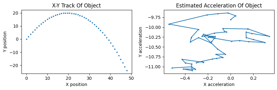
This gives us a good foundation for our object’s motion. But we’re ultimately interested in a stochastic process: \(\vec{x}(k) = F \vec{x}(k-1) + \vec{\eta}(k-1)\)

So let’s add noise \(\vec{\eta}(k) \sim \mathcal{N}(0,Q)\) to the process. We simplify/approximate a process noise covariance matrix that confines the variance to the acceleration components of the process:

# Approximate Q as only variance for the acceleration components ax and ay.
accel_var = 0.015
Q_true = np.array([
    [0, 0, 0, 0, 0, 0],
    [0, 0, 0, 0, 0, 0],
    [0, 0, accel_var, 0, 0, 0],
    [0, 0, 0, 0, 0, 0],
    [0, 0, 0, 0, 0, 0],
    [0, 0, 0, 0, 0, accel_var],
])

# Results matrix. Each row is the state for one timestep
true_xs = np.full((N, 6), np.nan)
true_xs[0,:] = x0

for k in range(1, N):
    # Process noise - only affects acceleration
    eta = rng.multivariate_normal(np.zeros(n), Q_true)
    
    true_xs[k, :] = F @ true_xs[k-1, :] + eta

fig, ax = plt.subplots(nrows=1, ncols=2, figsize=(9,3))
ax[0].plot(true_xs[:,0], true_xs[:,3], marker='o', linestyle='none', markersize=2)
ax[0].set_title('X-Y Track Of Object')
ax[0].set_xlabel('X position')
ax[0].set_ylabel('Y position')
ax[1].plot(true_xs[:,2], true_xs[:,5], marker='o', markersize=2)
ax[1].set_title('Estimated Acceleration Of Object')
ax[1].set_xlabel('X acceleration')
ax[1].set_ylabel('Y acceleration')
fig.tight_layout()
plt.show()

2.4.2. Synthesizing measurements

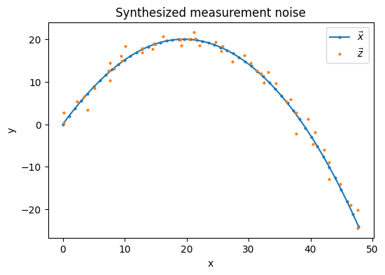
To synthesize our measurement series \(\vec{z}(k)\), we add bivariate white noise \(\vec{\xi}(k) \sim \mathcal{N}(0,R)\) to our synthesized true state series \(\vec{x}(k)\).

We will assume we only have positional sensors to take measurements, i.e. \(\vec{z}(k) = [z_x(k), z_y(k)]^T\). As there are no velocity or acceleration components to our measurements, \(\dot{x}\), \(\ddot{x}\), \(\dot{y}\), and \(\ddot{y}\) are all hidden variables ([Lab] Chpt. 5).

# Synthesize measurements by adding random noise to the true position series
z_var = 1.2
# Measurement (position) noise covariance matrix (independent bivariate normal)
R_true = np.array([
    [z_var, 0],
    [0, z_var],
])
zs = np.full((N, 2), np.nan)
zs[:, 0] = true_xs[:, 0] # x positions
zs[:, 1] = true_xs[:, 3] # y positions

zs = zs + rng.multivariate_normal(np.zeros(2), R_true, N)

plt.rcParams["figure.figsize"] = (6,4)
plt.plot(true_xs[:,0], true_xs[:,3], label=r'$\vec{x}$',  marker='o', markersize=2)
plt.plot(zs[:,0], zs[:,1], label=r'$\vec{z}$', marker='o', linestyle='none', markersize=2)
plt.title('Synthesized measurement noise')
plt.xlabel('x'); plt.ylabel('y')
plt.legend()
plt.show()

2.4.3. Multidimensional Filter Implementation

Now that we have our synthetic observations \(\vec{z}(k)\) we can apply a multivariate Kalman filter to obtain estimates \(\hat{x}(k)\) and do some analysis.

First we must implement that filter. The implementation below draws heavily from [Lab] Chpt. 6, extending that implementation to track 6 state variables instead of 2.

# Matrix H converts state vectors into measurement space
# In this model, that means grabbing the position values
H = np.array([
    [1, 0, 0, 0, 0, 0],
    [0, 0, 0, 1, 0, 0],
])

def kalman_6d(zs, R, Q, x_0, P_0):
    assert len(zs) == N
    # Store filter estimates (means and variances)
    xs = np.full((N, 6), np.nan)
    Ps = np.full((N, 6, 6), np.nan)
    
    # Initial estimate
    xs[0,:] = x_0
    Ps[0] = P_0
    
    x = np.copy(x_0)
    P = np.copy(P_0)

    # TODO: Should we exclude prediction calculation for first iteration?
    # But we still want to do the correction for the first iteration, right?
    for k in range(1, N):
        # 1) PREDICT
        prior = F @ xs[k-1,:]
        P = F @ P @ F.T + Q

        # 2) UPDATE
        # TODO: Currently using Labbe notation. Switch to Young?

        # Calculate system uncertainty
        S = H @ P @ H.T + R

        # Calculate kalman gain
        K = P @ H.T @ np.linalg.inv(S)

        # Calculate residual: Difference between prediction and measurement
        # (In measurement space)
        y = zs[k] - H @ prior

        # Caculate posterior state (corrected estimate and covar)
        post = prior + K @ y
        P = P - K @ H @ P

        # Save
        xs[k] = post
        Ps[k] = P
        
    return xs, Ps

# TODO: Known bug. When R and Q are zero matrices, the value of S's elements get tiny (floating
# point errors representing zero), which leads inv(S) to produce a matrix of nans. This produces
# nan estimates from that iteration onwards. Not sure how to avoid, but a workaround is to not pass
# in Q and R made of all zeros.

2.4.4. Demonstration on synthetic data

# Initialize filter state
# Guess the position somewhat accurately, leave the velocity and acceleration state guesses as 0
x_0 = np.array([1, 2, 0, 0.1, 0, 0])
P_0 = np.eye(6) * 50 # Start with very low confidence in predictions

# Assume we can configure the system's process and measurement noise params correctly
Q = Q_true
R = R_true

xs, Ps = kalman_6d(zs, R, Q, x_0, P_0)
    
# Extract covariances for position, velocity, and acceleration
pos_vars, vel_vars, acc_vars = utils.separate_covar_series(Ps)
    
# Plot track, measurements, and estimate for position
fig, ax = plt.subplots(figsize=(10,6))
ax.plot(true_xs[:,0], true_xs[:,3], label=r'$\vec{x}$',  marker='o', markersize=2)
ax.plot(xs[:,0], xs[:,3], label=r'$\hat{x}$',  marker='o', markersize=2)
ax.plot(zs[:,0], zs[:,1], label=r'$\vec{z}$', marker='o', linestyle='none', markersize=2)
ax.set_title('Kalman position estimate')
ax.set_xlabel('x position')
ax.set_ylabel('y position')
ax.legend()
plt.show()
glue('mv_kf_pos', fig, display=False)

# Plot track, measurements, and estimate for pos, vel, acc in a tight figure
fig, ax = plt.subplots(nrows=1, ncols=3, figsize=(10,3.5))
ax[0].plot(true_xs[:,0], true_xs[:,3], label=r'$\vec{x}$',  marker='o', markersize=2)
ax[0].plot(xs[:,0], xs[:,3], label=r'$\hat{x}$',  marker='o', markersize=2)
ax[0].plot(zs[:,0], zs[:,1], label=r'$\vec{z}$', marker='o', linestyle='none', markersize=2)
ax[0].set_title('Kalman position estimate')
ax[0].set_xlabel('x position')
ax[0].set_ylabel('y position')
ax[0].legend()
ax[1].plot(true_xs[:,1], true_xs[:,4], label=r'$\vec{x}$',  marker='o', markersize=2)
ax[1].plot(xs[:,1], xs[:,4], label=r'$\hat{x}$',  marker='o', markersize=2)
ax[1].set_title('Kalman velocity estimate')
ax[1].set_xlabel('x velocity')
ax[1].set_ylabel('y velocity')
ax[1].legend()
ax[2].plot(true_xs[:,2], true_xs[:,5], label=r'$\vec{x}$',  marker='o', markersize=2)
ax[2].plot(xs[:,2], xs[:,5], label=r'$\hat{x}$',  marker='o', markersize=2)
ax[2].set_title('Kalman acceleration estimate')
ax[2].set_xlabel('x acceleration')
ax[2].set_ylabel('y acceleration')
ax[2].legend()
fig.tight_layout()
plt.show()
glue('mv_kf_pos_vel_acc', fig, display=False)

# Plot positional variance
fig, ax = plt.subplots(nrows=1, ncols=3, figsize=(10,3.5))
ax[0].plot(np.arange(0,N), pos_vars[:,0,0], label=r'$\sigma_x$')
ax[0].plot(np.arange(0,N), pos_vars[:,1,1], label=r'$\sigma_y$')
ax[0].set_title('Position estimate variances')
ax[0].set_xlabel('t')
ax[0].set_ylabel(r'$\sigma^2$')
ax[0].legend()
ax[1].plot(np.arange(0,N), vel_vars[:,0,0], label=r'$\sigma_{\dot{x}}$')
ax[1].plot(np.arange(0,N), vel_vars[:,1,1], label=r'$\sigma_{\dot{y}}$')
ax[1].set_title('Velocity estimate variance')
ax[1].set_xlabel('t')
ax[1].set_ylabel(r'$\sigma^2$')
ax[1].legend()
ax[2].plot(np.arange(0,N), acc_vars[:,0,0], label=r'$\sigma_{\ddot{x}}$')
ax[2].plot(np.arange(0,N), acc_vars[:,1,1], label=r'$\sigma_{\ddot{y}}$')
ax[2].set_title('Acceleration estimate variance')
ax[2].set_xlabel('t')
ax[2].set_ylabel(r'$\sigma^2$')
ax[2].legend()
fig.tight_layout()
plt.show()
glue('mv_kf_pva_variances', fig, display=False)

# TODO could plot x and y pos, vel, and acc as functions of t.
# TODO Plot x(t) and vel_x(t) slopes overlaid

The covariance matrix \(P\) (for a given k):

\( P = \begin{bmatrix} \sigma_{x}^2 & \sigma_{x,\dot{x}}^2 & \sigma_{x,\ddot{x}}^2 & \sigma_{x,y}^2 & \sigma_{x,\dot{y}}^2 & \sigma_{x,\ddot{y}}^2 \\ \sigma_{\dot{x},x}^2 & \sigma_{\dot{x}}^2 & \sigma_{\dot{x},\ddot{x}}^2 & \sigma_{\dot{x},y}^2 & \sigma_{\dot{x},\dot{y}}^2 & \sigma_{\dot{x},\ddot{y}}^2 \\ \sigma_{\ddot{x},x}^2 & \sigma_{\ddot{x},\dot{x}}^2 & \sigma_{\ddot{x}}^2 & \sigma_{\ddot{x},y}^2 & \sigma_{\ddot{x},\dot{y}}^2 & \sigma_{\ddot{x},\ddot{y}}^2 \\ \sigma_{y,x}^2 & \sigma_{y,\dot{x}}^2 & \sigma_{y,\ddot{x}}^2 & \sigma_{y}^2 & \sigma_{y,\dot{y}}^2 & \sigma_{y,\ddot{y}}^2 \\ \sigma_{\dot{y},x}^2 & \sigma_{\dot{y},\dot{x}}^2 & \sigma_{\dot{y},\ddot{x}}^2 & \sigma_{\dot{y},y}^2 & \sigma_{\dot{y}}^2 & \sigma_{\dot{y},\ddot{y}}^2 \\ \sigma_{\ddot{y},x}^2 & \sigma_{\ddot{y},\dot{x}}^2 & \sigma_{\ddot{y},\ddot{x}}^2 & \sigma_{\ddot{y},y}^2 & \sigma_{\ddot{y},\dot{y}}^2 & \sigma_{\ddot{y}}^2 \end{bmatrix} \)

2.4.5. Exploring covariance of position with velocity

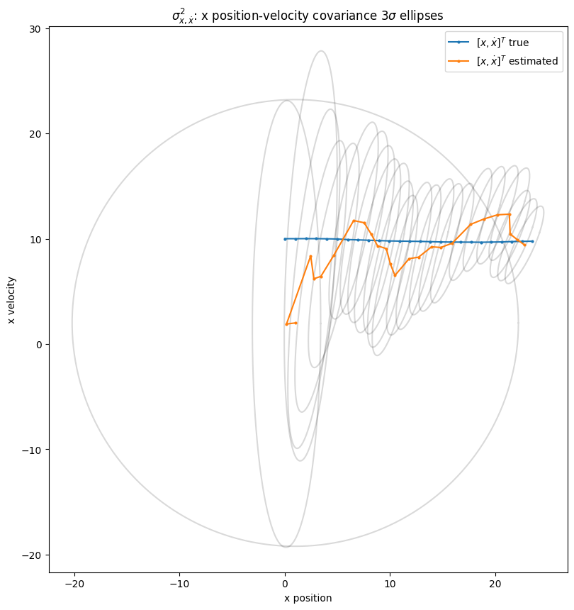
Below we see the \(3 \sigma\) ellipses for the covariance matrix of position with velocity \(\begin{bmatrix} \sigma_{x,x}^2 & \sigma_{x,\dot{x}}^2 \\ \sigma_{\dot{x},x}^2 & \sigma_{\dot{x},\dot{x}}^2 \end{bmatrix}\) in the \(x\)-dimension for first few timesteps.

The visualization displays how the filter learns the covariance between position and the hidden variable velocity over time. It starts with prediction uncertainty as a wide variance fully uncorrelated (circular) ellipse, then converges over time to the way it looks in the end: with a positive covariance between position and velocity.

# Extract pos-vel covariance in the x dimension
pos_vel_x_vars = np.full((N, 2, 2), np.nan)
for i in range(len(Ps)):
    P = Ps[i]
    pos_vel_x_vars[i] = np.array([[P[0,0], P[0,1]],[P[1,0], P[1,1]]])

# Plot
figure, axes = plt.subplots(1, figsize=(10,10)) 
axes.set_aspect(1) 

# Plot prediction 3-sigma covariance ellipses
steps = 25
for i in range(steps):
    S = pos_vel_x_vars[i]
    mu = np.array([xs[i,0], xs[i,1]])
    utils.plot_covar_ellipse(S, mu, alpha=0.15)
plt.plot(true_xs[:steps,0], true_xs[:steps,1], label=r'$[x,\dot{x}]^T$ true',  marker='o', markersize=2)
plt.plot(xs[:steps,0], xs[:steps,1], label=r'$[x,\dot{x}]^T$ estimated',  marker='o', markersize=2)
plt.title(r'$\sigma_{x,\dot{x}}^2$: x position-velocity covariance $3\sigma$ ellipses')
plt.xlabel('x position')
plt.ylabel('x velocity')
plt.legend()
plt.show()

2.4.6. Quantifying the Accuracy of the Kalman Filter’s Predictions

2.4.6.1. NEES (Normalized Estimated Error Squared)

NEES is one approach to quantifying the accuracy of the Kalman Filter’s estimates.

The NEES for time step \(k\) is \(\epsilon(k) = \tilde{x}(k)^T \textbf{P}^{-1} \tilde{x}(k)\), where the error vector \(\tilde{x}(k) = \vec{x}(k) - \hat{x}(k)\). Note this requires knowledge of the true state \(\vec{x}(k)\), which we have access to since we synthesized our input data.

In the below code, I

1. Calculate the NEES time series for my Kalman Filter implementation.

2. Show that this multidimensional filter implementation has a “good” average NEES score on my synthetic data (where “good” means the average NEES score is less than the dimension of the state vectors).

3. Numerically show that \(\epsilon(k)\) is chi-squared distributed with \(n\) degrees of freedom as is theoretically expected.

References: [Lab], [BSLK01]

xs_pos, xs_vel, xs_acc = utils.separate_state_series(xs)
true_xs_pos, true_xs_vel, true_xs_acc = utils.separate_state_series(true_xs)
Ps_pos, Ps_vel, Ps_acc = utils.separate_covar_series(Ps)

# Calculate the NEES series
def nees_series(true_xs, xs, Ps):
    x_tilde = true_xs - xs
    nees_ts = np.full(N, np.nan)
    for k in range(N): # TODO can we vectorize this loop?
        nees_ts[k] = x_tilde[k].T @ np.linalg.inv(Ps[k]) @ x_tilde[k]
    return nees_ts
        
# Calculate the mean NEES score
def mean_nees(true_xs, xs, Ps):
    nees_ts = nees_series(true_xs, xs, Ps)
    return np.mean(nees_ts)

## COMPLETE state vector NEES
fig, ax = plt.subplots(nrows=1, ncols=2, figsize=(9,3))
nees_ts = nees_series(true_xs, xs, Ps)
ax[0].plot(np.arange(0,N), nees_ts)
ax[0].set_title('Complete state NEES')
ax[0].set_xlabel('t')
ax[0].set_ylabel(r'$\vec{x},\dot{x},\ddot{x}$  NEES')

# Complete state NEES distribution compared to chi-2
domain = (np.floor(np.min(nees_ts)), np.ceil(np.max(nees_ts)))
# Set the number of histogram bins so each has width unity
num_bins = int(domain[1] - domain[0])
h_vals, bins = np.histogram(nees_ts, bins=num_bins, range=domain, density=True)
plt.bar(bins[:-1], h_vals)
domain_ls = np.linspace(domain[0],domain[1])
ax[1].plot(domain_ls, chi2.pdf(domain_ls, df=6), color='r', label=r'$\chi^2_6$')
ax[1].legend()
ax[1].set_xlabel(r'$\epsilon(k) values$')
ax[1].set_ylabel(r'density')
ax[1].set_title('Comparing numerical and theoretical distributions')
plt.tight_layout()
plt.show()

# A 'good' NEES score is: the average value of the NEES timeseries is less than the dimension of the state vector
print(f'Complete state mean NEES score: {mean_nees(true_xs, xs, Ps)}')

# POSITION NEES
# The difference between the estimate and the true position state
nees_ts = nees_series(true_xs_pos, xs_pos, Ps_pos)
fig, ax = plt.subplots(nrows=1, ncols=2, figsize=(9,3))
ax[0].plot(np.arange(0,N), nees_ts)
ax[0].set_title('Position state NEES')
ax[0].set_xlabel('t')
ax[0].set_ylabel(r'$\vec{x}$  NEES')

# Position NEES distribution compared to chi-2
domain = (np.floor(np.min(nees_ts)), np.ceil(np.max(nees_ts)))
# Set the number of histogram bins so each has width unity
num_bins = int(domain[1] - domain[0])
h_vals, bins = np.histogram(nees_ts, bins=num_bins, range=domain, density=True)
plt.bar(bins[:-1], h_vals)
domain_ls = np.linspace(domain[0],domain[1])
ax[1].plot(domain_ls, chi2.pdf(domain_ls, df=2), color='r', label=r'$\chi^2_2$')
ax[1].set_xlabel(r'$\epsilon(k) values$')
ax[1].set_ylabel(r'density')
ax[1].set_title('Comparing numerical and theoretical distributions')
ax[1].legend()
plt.tight_layout()
plt.show()
print(f'Position state mean NEES score: {mean_nees(true_xs_pos, xs_pos, Ps_pos)}')

# VELOCITY NEES
nees_ts = nees_series(true_xs_vel, xs_vel, Ps_vel)
fig, ax = plt.subplots(nrows=1, ncols=2, figsize=(9,3))
ax[0].plot(np.arange(0,N), nees_ts)
ax[0].set_title('Velocity state NEES')
ax[0].set_xlabel('t')
ax[0].set_ylabel(r'$\dot{x}$  NEES')

# ACCELERATION NEES
nees_ts = nees_series(true_xs_acc, xs_acc, Ps_acc)
ax[1].plot(np.arange(0,N), nees_ts)
ax[1].set_title('Acceleration state NEES')
ax[1].set_xlabel('t')
ax[1].set_ylabel(r'$\ddot{x}$  NEES')
plt.tight_layout()
plt.show()
print(f'Velocity state mean NEES score: {mean_nees(true_xs_vel, xs_vel, Ps_vel)}')
print(f'Acceleration state mean NEES score: {mean_nees(true_xs_acc, xs_acc, Ps_acc)}')

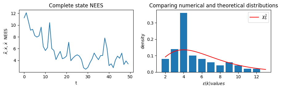
Complete state mean NEES score: 5.615083226038849

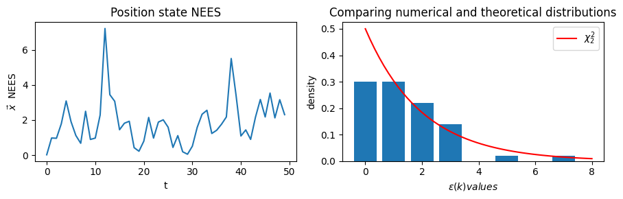
Position state mean NEES score: 1.8521419590449708

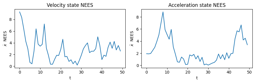
Velocity state mean NEES score: 2.893379246281296
Acceleration state mean NEES score: 2.503600489582321

Above we have shown:

• The full state vector \(\vec{x}\) (as well as the split out position, velocity, and accelerate state 2-tuples) comply with the \(\chi^2_k\) distributions, and that the average value of the NEES series is less than the number of elements in the respective state vector.

• The state vectors \(\epsilon(k)\) distributions are indeed \(\chi^2_k\), verified by overlaying the actual NEES values histogram with the \(\chi^2_k\) pdfs.

2.4.6.2. \(3\sigma\) Membership Accuracy Score: Do the true positions \(\vec{x}(k)\) fall within the \(\hat{x}(k)\) estimates’ \(3\sigma\) confidence ellipses?

# Return a boolean array, where each element encodes whether the k-th true
# state is within n-std confidence ellipse of the k-th estimate.
# Only works for 2D state
def within_confidence_ellipse(true_xs, xs, Ps, n_std=3.0):
    """
        Args: 
            xs: State estimate array
            true_xs: True state array
            Ps: Estimate covariance array
            n_std: Number of standard deviations defining the covar ellipse size
    """
    assert len(xs) == N
    assert len(xs[0]) == 2
    assert Ps[0].shape == (2,2)
    
    result = np.zeros(N, dtype=bool)
    for k in range(N):
        result[k] = utils.ellipse_contains(true_xs[k], xs[k], Ps[k], n_std=n_std)
    return result

def ratio_within_confidence_ellipse(true_xs, xs, Ps):
    accurate_ellipses = within_confidence_ellipse(true_xs, xs, Ps)
    return np.sum(accurate_ellipses) / len(accurate_ellipses)

# Visualize the accuracy of 2D state estimates as whether their 2x2 covariance ellipses
# contain the true state values.
def plot_3sig_membership_acccuracy(true_xs, xs, Ps, ax, n_std=3.0, xlabel='', ylabel=''):
    # Plot positional estimates with 3sigma ellipses
    ax.set_aspect(1) 

    # Plot estimated and true state
    plt.plot(true_xs[:,0], true_xs[:,1], label=r'$\vec{x}$',  marker='o', markersize=2, linestyle='none')
    plt.plot(xs[:,0], xs[:,1], label=r'$\hat{x}$',  marker='o', markersize=2)

    # Plot estimates' 3-sigma elipses
    for k in range(N):
        utils.plot_covar_ellipse(Ps[k], xs[k], alpha=0.15)

    # Calculate whether k-th true value falls within k-th estimates ellipse
    accurate_ellipses = within_confidence_ellipse(true_xs, xs, Ps, n_std=3.0)

    # Plot line segments connecting each estimate to its true value for time k
    line_segs = []
    for k in range(N):
        line_segs.append([xs[k], true_xs[k]])

    # Color line segments based on the estimate accuracy
    colors = np.where(accurate_ellipses, 'green', 'red')

    lc = mc.LineCollection(line_segs, linewidths=1.5, linestyle='solid', colors=colors, label=r'$|\vec{x}-\hat{x}|$')
    ax.add_collection(lc)

    plt.title(r'$3 \sigma$ Membership Accuracy')
    plt.xlabel(xlabel)
    plt.ylabel(ylabel)
    plt.legend()
    plt.show()
    print(f'Percent of estimate covar ellipse containing true state: {np.sum(accurate_ellipses)*100/N:.02f}%')
    
# Demonstrate with x-y position state estimates
Q_scale = 5.0
R_scale = 0.25
Q = Q_true * Q_scale
R = R_true * R_scale

print(f'Q * {Q_scale:.01f}.  R * {R_scale:.01f}.')

# Run Kalman filter for (Q,R) combo
P_0 = np.eye(6) * 50 # Start with very low confidence in predictions
v_0 = np.array([5., 0, 0, 5, 0, 0]) # Start with an ok initial state
xs, Ps = kalman_6d(zs, R, Q, v_0, P_0)

xs_pos, _, _ = utils.separate_state_series(xs)
true_xs_pos, _, _ = utils.separate_state_series(true_xs)
Ps_pos, _, _ = utils.separate_covar_series(Ps)
fig, ax = plt.subplots(1, figsize=(8,8))
plot_3sig_membership_acccuracy(true_xs_pos, xs_pos, Ps_pos, ax=ax, n_std=3.0, 
                     xlabel='x position', ylabel='y position')
glue('3sig_membership_viz', fig, display=False)

ratio = ratio_within_confidence_ellipse(true_xs_pos, xs_pos, Ps_pos)
glue('3sm_ratio', ratio, display=False)

print(f'R:\n{R}\nQ:\n{Q}')

Q * 5.0.  R * 0.2.

Percent of estimate covar ellipse containing true state: 80.00%

R:
[[0.3 0. ]
 [0.  0.3]]
Q:
[[0.    0.    0.    0.    0.    0.   ]
 [0.    0.    0.    0.    0.    0.   ]
 [0.    0.    0.075 0.    0.    0.   ]
 [0.    0.    0.    0.    0.    0.   ]
 [0.    0.    0.    0.    0.    0.   ]
 [0.    0.    0.    0.    0.    0.075]]

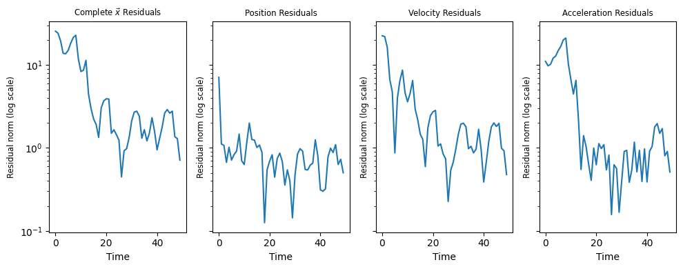
2.4.6.3. Exploring Residuals

Another simple way to gain intuition about the filter’s accuracy is to visualize the residuals \(\vec{x}(k)-\hat{x}(k)\), or their norms:

# rs = true_xs - xs
# Note this function assumes the given ax is part of a multi subplot figure
def plot_residuals(ax, rs, title=''):
    rs_norms = np.full(N, np.nan)
    for i in range(N):
        rs_norms[i] = np.linalg.norm(rs[i])
    t = np.arange(0,N)
    ax.set_yscale('log')
    ax.plot(t, rs_norms)
    ax.set_title(title, fontsize='small')
    ax.set_xlabel('Time')
    ax.set_ylabel('Residual norm (log scale)', fontsize='small')

# Calculate and plot residuals for multiple (track, estimate) pairs on one figure
def plot_all_residuals_2(tracks, estimates):
    """
    Args:
        tracks: List of true state timeseries
        estimates: List of estimated state timeseries
    """
    fig, axs = plt.subplots(nrows=1, ncols=4, sharex=True, sharey=True, figsize=(10,4))
    
    for track, estimate in zip(tracks, estimates):
        xs_pos, xs_vel, xs_acc = utils.separate_state_series(track)
        true_xs_pos, true_xs_vel, true_xs_acc = utils.separate_state_series(estimate)

        # Complete Residuals
        rs = track - estimate
        plot_residuals(axs[0], rs, title=r'Complete $\vec{x}$ Residuals')

        # Position residuals
        rs = true_xs_pos - xs_pos
        plot_residuals(axs[1], rs, title='Position Residuals')

        # Velocity residuals
        rs = true_xs_vel - xs_vel
        plot_residuals(axs[2], rs, title='Velocity Residuals')

        # Velocity residuals
        rs = true_xs_acc - xs_acc
        plot_residuals(axs[3], rs, title='Acceleration Residuals')
    
    plt.tight_layout()
    plt.show()

plot_all_residuals_2([true_xs], [xs])

2.4.7. Visualizing the \(3 \sigma\) membership accuracy score as a function of initial state guess perturbation

d = len(xs[0])
num_incr = 20
samples_per_incr = 100

# For each initial state guess perturbation scale, we'll track the 3-sigma membership
# accuracy score.
accuracy_3sm = []
accuracy_nees = []

# For p in a set of increasing distances (relative scale to true x0's norm)
for p in np.linspace(0.0, 20.0, num=num_incr):    
    # Generate random initial state vectors perturbed by p from true initial state x0
    # via the Muller method.
    x0_norm = np.linalg.norm(true_xs[0])
    r = x0_norm * p
    init_points = np.full((samples_per_incr, d), np.nan)
    for i in range(samples_per_incr):
        init_points[i] = utils.random_point_on_dsphere(r=r, d=d, v0=true_xs[0])

    # Run Kalman filter and check accuracy for each initial (position) state guess
    for v_0 in init_points:
        P_0 = np.eye(6) * 50 # Start with very low confidence in predictions
        xs, Ps = kalman_6d(zs, R, Q, v_0, P_0)
        xs_pos, _, _ = utils.separate_state_series(xs)
        true_xs_pos, _, _ = utils.separate_state_series(true_xs)
        Ps_pos, _, _ = utils.separate_covar_series(Ps)
        ratio = ratio_within_confidence_ellipse(true_xs_pos, xs_pos, Ps_pos)
        accuracy_3sm.append((p, ratio))
        # TODO Calculate accuracy ratios for velocity and acceleration also?
        # Calculate mean NEES score
        accuracy_nees.append((p, mean_nees(true_xs_pos, xs_pos, Ps_pos)))
        
accuracy_3sm = np.array(accuracy_3sm)
accuracy_nees = np.array(accuracy_nees)
assert len(accuracy_3sm) == num_incr * samples_per_incr

# Calculate mean accuracy score for each perturbation scale value
# Had to do so manually because I couldn't get np's 2D Histogram working
x_vals = np.unique(accuracy_3sm[:,0])
avg_y_vals_3sm = np.zeros(len(x_vals))
avg_y_vals_nees = np.zeros(len(x_vals))
d_3sm = dict(zip(x_vals, [[] for i in range(len(x_vals))]))
d_nees = dict(zip(x_vals, [[] for i in range(len(x_vals))]))
for i in range(len(accuracy_3sm)):
    p, score_3sm = accuracy_3sm[i]
    d_3sm[p].append(score_3sm)
    p, score_nees = accuracy_nees[i]
    d_nees[p].append(score_nees)
for i in range(len(x_vals)):
    x = x_vals[i]
    y_vals_3sm = d_3sm[x]
    avg_y_vals_3sm[i] = np.mean(y_vals_3sm)
    y_vals_nees = d_nees[x]
    avg_y_vals_nees[i] = np.mean(y_vals_nees)

# Plot 3-sigma membership accuracy vs perturbation scale
fig, ax = plt.subplots(figsize=(8,5))
ax.scatter(accuracy_3sm[:,0], accuracy_3sm[:,1], s=1, alpha=0.2)
ax.plot(x_vals, avg_y_vals_3sm, color='green', label='Avg. Accuracy')
ax.set_xlabel("Initial State Guess Perturbation Scale")
ax.set_ylabel(r"$3 \sigma$ Membership Accuracy Score")
ax.set_title("$3 \sigma$ Membership Accuracy vs. Perturbation Scale")
ax.legend()
plt.show()
glue('3sm_v_perturbation', fig, display=False)

# Plot NEES mean accuracy vs perturbation scale
fig, ax = plt.subplots(figsize=(8,5))
ax.scatter(accuracy_nees[:,0], accuracy_nees[:,1], s=1, alpha=0.2)
ax.plot(x_vals, avg_y_vals_nees, color='green', label='Avg. Accuracy')
ax.set_xlabel("Initial State Guess Perturbation Scale")
ax.set_ylabel(r"Mean NEES Accuracy Score")
ax.set_title("Mean NEES Accuracy vs. Perturbation Scale")
ax.legend()
plt.show()
glue('nees_v_perturbation', fig, display=False)

2.4.8. Exploring \(Q\),\(R\) parameter space for the multivariable Kalman filter example

In our initial exploration, we assumed we could configure the filter’s \(Q\) and \(R\) values perfectly (i.e. to the noise values that were used to generate the synthetic data). But what about the more realistic scenario where we don’t know the true \(Q\) and \(R\) values?

Let \(Q*\) and \(R*\) be the true process and measurement noise covariance matrices, respectively. Below we explore tuning \(Q\) and \(R\) (the parameters passed to the filter) covariance matrices to an increasing range of scaling factors applied to \(Q*\) and \(R*\). For each point in our (\(Q\),\(R\)) parameter space, we run the Kalman filter on the synthetic data set and evaluate its accuracy (via both metrics):

# Run the kalman filter and compute the both the 3sigma membership and NEES accuracy
# scores for position state estimates for the given Q_scale and R_scale factor
def calc_accuracy_scores(Q_scale, R_scale):
    Q = Q_true * Q_scale
    R = R_true * R_scale

    # Run Kalman filter for (Q,R) combo
    P_0 = np.eye(6) * 50 # Start with very low confidence in predictions
    v_0 = np.array([5., 0, 0, 5, 0, 0]) # Start with an ok initial state
    xs, Ps = kalman_6d(zs, R, Q, v_0, P_0)

    xs_pos, _, _ = utils.separate_state_series(xs)
    true_xs_pos, _, _ = utils.separate_state_series(true_xs)
    Ps_pos, _, _ = utils.separate_covar_series(Ps)
    assert len(xs_pos[0]) == 2

    # Calculate accuracy scores
    accuracy_3sm = ratio_within_confidence_ellipse(true_xs_pos, xs_pos, Ps_pos)
    accuracy_nees = mean_nees(true_xs_pos, xs_pos, Ps_pos)

    return (accuracy_3sm, accuracy_nees)

# Iterate through the (Q,R) parameter space 
# In terms of percentages of the true param values
num_iters = 20

# The Q and R matrices are simple, they can be represented by their top left corner
# i.e. the variance of the x position
Q_scales = np.linspace(10**-6, 5.0, num=num_iters)
R_scales = np.linspace(10**-1, 1.2, num=num_iters)

# Meshgrid it and calculate surface of accuracy scores (for both 3sigma membership and NEES)
QQ_scales, RR_scales = np.meshgrid(Q_scales, R_scales)
accuracy_scores = np.vectorize(calc_accuracy_scores)(QQ_scales, RR_scales)
scores_3sm, scores_nees = accuracy_scores[0], accuracy_scores[1]

# Plot 3-sigma membership accuracy score surface and contour map
#fig = plt.figure(figsize=plt.figaspect(0.5))
fig = plt.figure(figsize=(8.5,4))
ax = fig.add_subplot(1, 2, 1, projection='3d')
ax.plot_surface(QQ_scales, RR_scales, scores_3sm, cmap='viridis')
ax.set_box_aspect(aspect=None, zoom=0.85)
ax.set_xlabel('Q Scale')
ax.set_ylabel('R Scale')
ax.set_zlabel(r'Accuracy')
ax.set_title(r'$3 \sigma$ Membership Score vs.' "\n"
             '(Q,R) Perturbation Scale')
        
# Plot mean NEES accuracy score surface
ax = fig.add_subplot(1, 2, 2, projection='3d')
ax.plot_surface(QQ_scales, RR_scales, scores_nees, cmap='viridis')
ax.view_init(elev=20, azim=30, roll=0)
ax.set_box_aspect(aspect=None, zoom=0.85)
ax.set_xlabel('Q Scale')
ax.set_ylabel('R Scale')
ax.set_zlabel('Accuracy')
ax.set_title(r'NEES Membership Score vs.' "\n"
             '(Q,R) Perturbation Scale')
plt.tight_layout()
plt.show()
glue('acc_surface_fig', fig, display=False)